Python

【Python】scikit-learnを使ってみた

データは昭和電業社の「モータ制御開発 支援システム Simtrol-m」から
まぁこんなデータなわけです

普通のPID制御なんですが、これを学習させて実測値に近いシミュレートをしようという魂胆です
具体的には、
比例定数と積分定数、微分定数を突っ込めば、電流、電圧、回転数が出るよというものを目指します。

と書きましたが諸事情によりとりあえず積分定数のみ

import csv
import os
from sklearn.tree import DecisionTreeRegressor
import matplotlib.pyplot as plt
import numpy as np

train_X = []
train_Y = []
test_X = [[] for i in range(6)]
test_Y = [[] for i in range(6)]
filepathS = ["*:\*******\****.csv", \
             "*:\*******\****.csv", \
             "*:\*******\****.csv", \
             "*:\*******\****.csv", \
             "*:\*******\****.csv", \
             "*:\*******\****.csv"]

for a,filepath in enumerate(filepathS):
    basename = os.path.basename(filepath)
    basename = basename[:-4]
    basename = basename.split("d")

    ConstInteg = float(basename[1])
　　
　　#csv読み込み
    csv_file = open(filepath, "r", encoding="ms932", errors="", newline="" )
    f = csv.reader(csv_file, delimiter=",", doublequote=True, lineterminator="\r\n", quotechar='"', skipinitialspace=True)

    i = 0
    for row in f:
        if i > 5 :
            print(row)

            train_X.append([ConstInteg,float(row[0])])
            train_Y.append([float(row[2]),float(row[3]),float(row[4])])

            test_X[a].append([ConstInteg,float(row[0])])
            test_Y[a].append([float(row[2]),float(row[3]),float(row[4])])

        i += 1

clf = DecisionTreeRegressor()
# 学習させる
clf.fit(train_X, train_Y)

print(clf.score(train_X, train_Y))

# -----------------------------------------------------
# 以下、結果

ConstantOfIntegration = 3.8

test_X1 = []
for b in test_X[1]:
    test_X1.append([ConstantOfIntegration,b[1]])

result = clf.predict(test_X1)

# 以下グラフ用
result = np.array(result)
test_X = np.array(test_X)

x = test_X[0][:,[1]]
y1 = result[:,[0]]
y2 = result[:,[1]]
y3 = result[:,[2]]

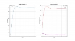
fig, (axL, axR) = plt.subplots(ncols=2, figsize=(22,12))

axL.plot(x, y1, label='(rpm)')
axL.set_title("Constant of Integration = "+str(ConstantOfIntegration))
axL.set_xlabel('time[s]')
axL.set_ylabel('Rotational speed')
axL.grid(True)

y_2000 = []
for c,yy1 in enumerate(y1):
    if yy1 >= 2000:
        y_2000.append(x[c])

axL.legend(title='2000rpm>= '+str(y_2000[0]), loc='upper left')

axR.plot(x, y2, label='(V)', color='r')
axR.plot(x, y3, label='(A)', color='m')
axR.set_title("Constant of Integration = "+str(ConstantOfIntegration))
axR.set_xlabel('time[s]')
axR.set_ylabel('Voltage / Intecity of Current')
axR.grid(True)
axR.legend(title='Vmax = '+str(max(y2))+'\nAmax = '+str(max(y3)))

plt.show()

シリアライズはしてません。

実行結果がこちら

学習データの範囲内ならそこそこの精度？
scikit-learn万歳!!
もっと学習用のデータが欲しい!!

by MSAdoti